VLOOKUP Tutorial: Updating prices in a master price list

MVP Bill Jelen has created this VLOOKUP tutorial for those of you who have a basic working knowledge of Excel but want to improve your skills. This tutorial assumes you’ve heard about the VLOOKUP function and its benefits, but that you don’t really know how or when you might use it.  Bill uses the example of updating prices in a product list to introduce the value of this time-saving function.

The Problem: It’s taking way too long to find and update prices in a master price list

• Attempt 1: Use CTRL + F to update the list
• Attempt 2: Use Find All to update the list

The Problem: It’s taking way too long to find and update prices in a master price list

Suppose that you maintain an Excel workbook with over 10,000 prices for products that your company sells. Parts are arranged in sections by category. You have part numbers in column A, prices in column B, and other information in column C. Now, imagine that your manager just gave you a worksheet with updates for 475 of the items in your list.

Attempt 1: Use CTRL + F to update the list

You decide to copy the price update to a blank section of your master price list.

From this point, you start trying to find each item from the new list in the old list. Since the items in the old list are not sorted and cannot easily be sorted across the various sections of the price list, you decide to use the Find command to make the process easier.

Here is your first attempt:

1. Select the first part number from the new list in cell G3
2. Press Ctrl+C to copy this item to the clipboard
3. Select all of column A by clicking on the A heading
4. Press Ctrl+F to open the Find dialog
5. Press Ctrl+V to paste the part number into the Find dialog
6. Click the Find button

You are now at row 2063 and fairly proud that you didn’t have to click PgDn one hundred times to get here. Unfortunately, you’ve forgotten the new price so you have to start over.

Attempt 2: Use Find All to update the list

You try jotting the new price on a sheet of scrap paper, but then you think there might be a faster way. After some experimenting, you end up with this awesome set of steps:

1. Select the next part number from the new list (you are down to G9) by now.
2. Press Ctrl+C to copy that cell to the clipboard
3. Press Ctrl+A twice to select all cells in the worksheet
4. Press Ctrl+F to open the Find dialog
5. Press Ctrl+V to paste the part number in the Find dialog
6. Press Alt+A to Find All! This brings up a list of both the item in the original list and the item in the new list
7. Switch between the two cells using the up and down arrow keys.
8. At this point, it is probably easier to switch to the mouse. Click on the new price. Right-click and choose Copy. Click on the old price. Right-click and choose paste.
9. You can return to the right section of the new price list using the hyperlinks in the still-open Find dialog.

Even with this improved set of steps, it is taking almost 1 minute per item. You do some quick math and realize that 450 items are going to require 8 mind-numbing hours. Your first thought might be, “There has to be a better way, but what is it?”

The Solution: Speed up the process with VLOOKUP

I began working as a financial analyst in 1989. I’ve learned that data is rarely perfect.

This price list workbook is a case in point. It has been handed down in your department for the last dozen years. It was set up by some guy named Bob who no longer works here. In the workbook, there are lots of things that would have made life easier.

For example, it would have been nice if:

• The category information was in another column, so you could easily sort the list by part number and then back by category.
• The list of new prices included all the items where the price did not change, and if it was in the exact same order as your list, so you could copy and paste huge ranges of prices.
• Your manager would have just done this himself.

But, in real life, data is not perfect. When data is not perfect, knowing an Excel function called VLOOKUP can save the day.

VLOOKUP explained

VLOOKUP stands for “Vertical Lookup.” The vertical means that your list of new prices is going down the spreadsheet instead of across. (If you are wondering, there is an HLOOKUP for when your lookup table is going across.)

The tooltip for VLOOKUP says you need:

=VLOOKUP(lookup_value,table_array,col_index_number,[range_lookup])

• Lookup_value is the part number that you are looking up. To find a new price for the part number in A2, you are looking for A2. =VLOOKUP(A2,
• Table_array is the lookup table. The data that you are looking to match must be in the first column of the lookup table. That works in this case, because part number is in column G and new price is in column H. If those had been reversed, you would copy the prices so they are to the right of the part numbers. When you type the address of the table, make sure to use dollar signs so that the table reference doesn’t change as you copy the formula down your worksheet. Instead of G3:H477, use $G$3:$H$477. Those dollar signs tell Excel to not lower the range as the formula gets copied down. =VLOOKUP(A2,$G$3:$H$477,
• Col_index_number tells Excel which column you want to return from the lookup table. In this case, you only have two columns. Part number is in the first column of the lookup table. New Price is in the second column of the lookup table. Since you want to return New Price, use 2 for the column. =VLOOKUP(A2,$G$3:$H$477,2
• Range_lookup – the square brackets in the tooltip say that this argument is optional, but in real life it is not optional! You should always put False as the fourth argument. If you leave the argument off, you are allowing Excel to find close matches. Close matches are never appropriate when you are doing the type of lookup described in this situation. =VLOOKUP(A2,$G$3:$H$477,2,False)

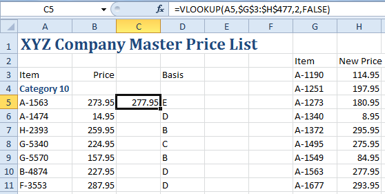
Add a new column to your price list called New Price. Enter =VLOOKUP(A2,$G$3:$H$477,2,False) in cell C5. You get the new price. This looks promising!

Your first VLOOKUP returns the new price

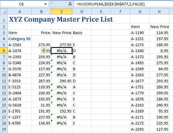
Select the formula in C5 and double-click the fill handle to copy the formula down. (The fill handle is the square dot in the bottom right corner of the selected cell.) Because of the blank cells between categories, the fill handle will only copy the formula down to the end of the first category. Already, you can see that something seems to be wrong.

Uh-oh! #N/A errors are usually bad, but maybe not in this case

Techniques for dealing with inevitable #N/A errors

A few of the VLOOKUP formulas are returning numbers. Many more are returning the #N/A error. When you do a VLOOKUP, the #N/A error means that the value you are looking up is not found in the lookup table. In this case, this is to be expected, since only 475 of the 10,000 prices are being updated.

Since you are expecting the #N/A errors, you can use the IFERROR function (available in Excel 2007 or later) to replace the #N/A with something else. You might put a space. You might put a zero. Or…in this case, if you don’t have a new price, then the old price is still valid, so you could put the old price!

Edit the original formula in C5. Here are the three formulas you could use:

• To show a blank, use =IFERROR(VLOOKUP(A5,$G$3:$H$477,2,FALSE),””)
• To show a zero, use =IFERROR(VLOOKUP(A5,$G$3:$H$477,2,FALSE),0)
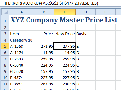
• To use the old price, use =IFERROR(VLOOKUP(A5,$G$3:$H$477,2,FALSE),B5)

Choose a formula and copy it down. Your new column shows the new price if there is one, and the old price if there isn’t one.

 =IFERROR() to the rescue

In this video, see how I define VLOOKUP and explain the VLOOKUP formula, and get rid of #N/A:

Use conditional formatting to highlight new prices

When I look at the two columns of data, it is hard to see which prices changed and which did not. You can use conditional formatting to highlight which items changed.

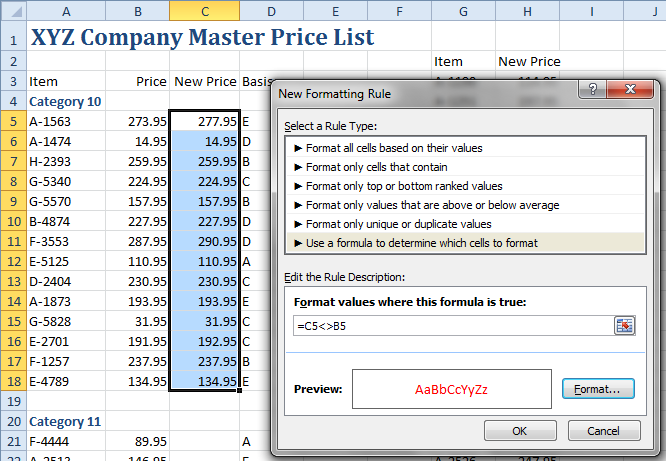
1. Select C5:C18. Although you are formatting a large range of cells, you need to do the following steps thinking only about the first cell in the range, C5.
2. Select Home, Conditional Formatting, New Rule.
3. Choose Use a Formula to Determine Which Cells to Format
4. In the rule description, type a formula of =C5<>B5
5. Click the Format button. Choose a red font. The dialog will look like Figure 4.
6. Click OK to apply the conditional format.

Any prices that have changed will appear in red.

Pain is relative: Copy your VLOOKUP formula to other categories

So far, you’ve solved the problem for a very small category of the master price list. You need to copy the C5 cell to the first row of the next category and use the fill handle to fill down. With 10 more categories, you will repeat this process several times and it might take 5 minutes to perform the copy operation repeatedly. Maybe it would be easier to copy all the way down to row 10000 and then manually clear out the blank rows between the categories. Someday you should reorganize the spreadsheet, but for today, you’ve save a lot of time.

Don’t forget: Change those formulas to values before you delete the new price range

At this point, you decide you don’t need the temporary range over in G:H any more. Don’t delete it yet! Those VLOOKUP formulas back in column C are still using that range. You need to convert the formulas to values.

1. Select all of column C
2. Right-click and choose Copy
3. Right-click and choose the 123 icon for Paste Values

I’m Speechless

If you’ve followed along here, you might not know what to say. You might be upset that you wasted so much time using the Find method and wasted one day of your life every month for the last 18 months. You might be angry that you never knew about VLOOKUP before. You might be giddy that you solved this problem in 20 minutes instead of 8 hours. (And…once you gain more confidence with VLOOKUP, you’ll be able to solve the problem faster and faster each month.) You might be plotting what you can do with all the time you just got back today (“long lunch!”).

VLOOKUP solved this cool problem and can solve many more problems.

When you were manually finding the items, it was natural to start with the shorter list of 475 items with the intent to work through it. Since VLOOKUP is incredibly fast, you can throw the VLOOKUP at all 10,000 items and let the IFERROR clean up the unfound entries.

Many people get discouraged when they encounter the #N/A errors from VLOOKUP. Understand that some #N/A are to be expected. It is part of the messiness of data in real life.

What to do with your free time–perform a quick quality-check

Have you done this process manually in the past? Did the part numbers in the new price list match up correctly? As a human, you would recognize “A-1234” and “A1234” to likely be the same item, but VLOOKUP will not understand this. Take an extra five minutes to make sure that all of the items in your new price list are found in the original table:

1. Add a column heading in I2 called “Is it OK?”
2. The formula in I3 is =VLOOKUP(I3,A:A,1,False). This formula will look for the part number from I3 over in column A. If it is found, it will return the first column of the lookup table, which is the part number from column A. If it is not found, it will return #N/A.
3. Copy that formula down by double-clicking the fill handle.
4. Sort descending by column I. Select one cell such as I2 and click the ZA button on the data tab. If there are any #N/A values that come to the top of the list, it means that the part number in I is not found in column A.
5. Do some research on these. Are they mis-typed? Are they new?

This is just one example of the many ways to use VLOOKUP. Check out vlookupweek.wordpress.com for many additional articles on other ways to use VLOOKUP.