Beyond column filters: Slicers on tables

This blog post is brought to you by John Campbell, Lead Program Manager for the Excel Web App team.

Slicers were first introduced in Excel 2010 and made filtering PivotTables as simple as clicking a button. We’ve taken the goodness of slicers but moved it beyond just PivotTables – with Excel 2013 you can now create slicers on any table! And, as you’ll see in throughout this article, all of this works in a browser too using Excel Web App.

Since Halloween is coming up soon, I’ve whipped up a small data set showing some great Horror novels to help you get into a spooky mood. When deciding which books you might want to read, you could use the existing filter drop downs on the table columns and peck your way through. For this example data set, since it is so small, that would probably work fine. But let’s see how much better the experience could be if we added some slicers.

Here’s the starting table of data (brought to you via embedding this table with Excel Web App):

Insert slicers

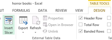
Let’s get some slicers inserted! The first thing to do is to select the table (any cell in the table will do), and then click the Insert Slicers button from the Design tab of the Table Tools ribbon.

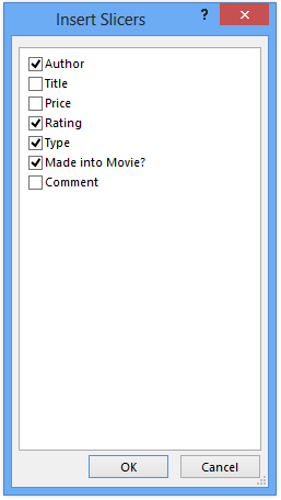
Now you’ll get a dialog asking you which columns you want to create slicers for. Each slicer filters a single column of data and you can create slicers on any column you like. For this example, let’s go ahead and select the checkboxes for the following columns: Author, Rating, Type, and Made into Movie.

That will create the slicers and drop them in your workbook. Go ahead and drag them all next to the left side of the table. You’ll now have some basic slicers that you can use to filter the table.

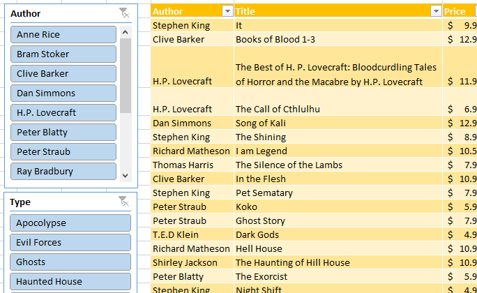
Go ahead and click the slicer buttons and watch your table filter – try finding books by your favorite author, by the type of monster you like, etc.

Here are a few things to note as you filter:

• The table column filter buttons show the same “filtered state” as the slicers. That’s because under the covers they work the same way. So you can use the table drop down filters and the slicers together (this can be useful in more advanced filtering scenarios).
• The slicer buttons themselves tell you about your data. For instance if you select Peter Straub from the authors slicer, you’ll see that while there is data in our list for lots of types of books, he only has books about Ghosts or Psychopath in our list, with ratings that are either 4 or 4.5, and some of his books have been made into movies.

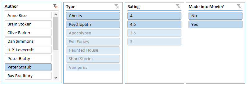
• The slicers are additive – that is you can keep applying more filters as you go. So if you click Ghosts on the Type slicer, then you’ll see there’s only 4.5 rated books written by Peter Straub about ghosts and it was made into a movie. And if you look at your table you’ll see the book shown there (it turns out there’s only one).

• The slicer buttons update as you type new data into the table. Go ahead and change the rating from 4.5 to 5 and note that the slicers update in real time.
• You can select multiple buttons via clicking and dragging, Shift + click, or Ctrl + click.
• Slicers are “floating” objects in Excel – that means you can put them anywhere you want to deliver the best reporting experience. For instance, you may create a chart based off your table and just want to show the chart. No problem – add your slicers on the table columns you want, and then just put the slicers next to your chart. People don’t even need to see your table – as you use the slicers you’ll see your chart update in real time.

Go ahead and click the Clear Filter icon on the top right of your slicers so you can see the whole table again.

Make it look and work great

Let’s customize the slicers and make the report look a little nicer, and show of some of the other slicer capabilities along the way.

Move the Rating and Made into Movie slicers to the top of the table and make it smaller and wider (you can use the grab handles to easily control the sizing).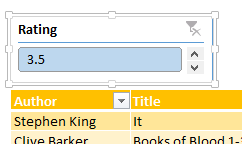

Customize the slicer look and feel

Select the Ratings slicer. Now on the Buttons chunk of the Options tab of the Slicer Tools ribbon, go ahead and set it to 4 columns. And while you’re at it, go ahead and apply a light orange style so it better matches our table (in fact, do this with all your slicers).

Note that slicers are highly customizable – you can control the specific height and width of buttons, along with the styles, individual highlights of buttons, and even more advanced things like hiding buttons that have no data – feel free to play around with the different options and settings dialogs you can find from that ribbon.

Focus on the relevant data – without losing the ability to filter

As is often the case with data, and this is way more common with large data sets where you might be filtering something like sales data by country, the filters are best as filters and you don’t always need to see them in the table of data. For instance, we have all the author, type, and rating information in our slicers now. Those values are most useful to us as filters and are redundant in the table.  So let’s go ahead and hide those columns – just right click on columns E, H, I, and J, and hide them.

This now takes a wider table and makes it narrower and easier to read – all without losing any of the data or your ability to filter it!

And lastly, you can now turn off the drop downs on table column headers without losing the ability to filter. Select the table (any cell in the table will do) and deselect the Filter Button checkbox on the Table Style Options chunk of the Table Tools Design ribbon.

This will give your table a nice crisp appearance in cases where you don’t need the sort/filter options from the drop down menu. In the past you would have to turn off all the filtering capability to do this, but with slicers on tables you can now have your cake and eat it too.

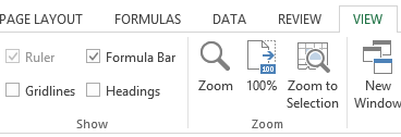
Finally, to tighten things just a bit more, from the Show chunk of the View tab on the ribbon, turn off Gridlines and Headings.

You should now have a nice crisp and clean report that looks something like this:

Wrapping up

Slicers are simple, powerful, and customizable controls that you can use to drive your Excel reports – and with Excel 2013, slicers have extended their reach to include tables. And with Excel Web App, you can take those reports and share them widely.

At first glance they might just seem like a straight duplication of the existing table filter drop downs. But take a closer look because you can go beyond what table column row filters can do. While they do the same type of filtering they open the door and allow you to do things like:

• Improve the UI of your report by turning off the filter buttons on table headers
• Hide columns you don’t need while still being able to use them to filter – this makes for narrower, cleaner tables
• Surface more important filters as buttons to make them stand out from the rest of the table
• Create more focused reports – since they are floating objects you can put them next to the interesting part of the spreadsheet you want your users to see – your chart, report summary, etc. Tabular data is great, but isn’t always what you want to show.

There’s a bunch of stuff I didn’t cover about slicers on tables – some of the more advanced things include smart update behavior of slicers when the data set is very large, using slicers on query tables, or how slicers work in Gallery view on Excel Web App – but those are topics for another day.

Feedback – we want to hear from you!

Thoughts? Concerns? Things you love about slicers? Things you would like to see slicers do in the future? We want to hear from you and look forward to any comments you have on this article!