Time grouping enhancements in Excel 2016

Excel 2016 introduces new features and improvements that help you streamline your data analysis. Today we will walk through the new options for building PivotTables with a Date/Time column and show how to surface time-based insights in your data. Additionally, we will help you take advantage of the ability to navigate your PivotCharts using drill-down buttons.

Automatic time grouping

Automatic time grouping, a new feature in Excel 2016, helps use time-related fields in a PivotTable by auto-detecting and grouping them on your behalf. The automatic grouping creates new Date/Time columns and automatically populates the PivotTable in one action. This allows users to quickly start analyzing their data across different levels of time with drill-down capabilities.

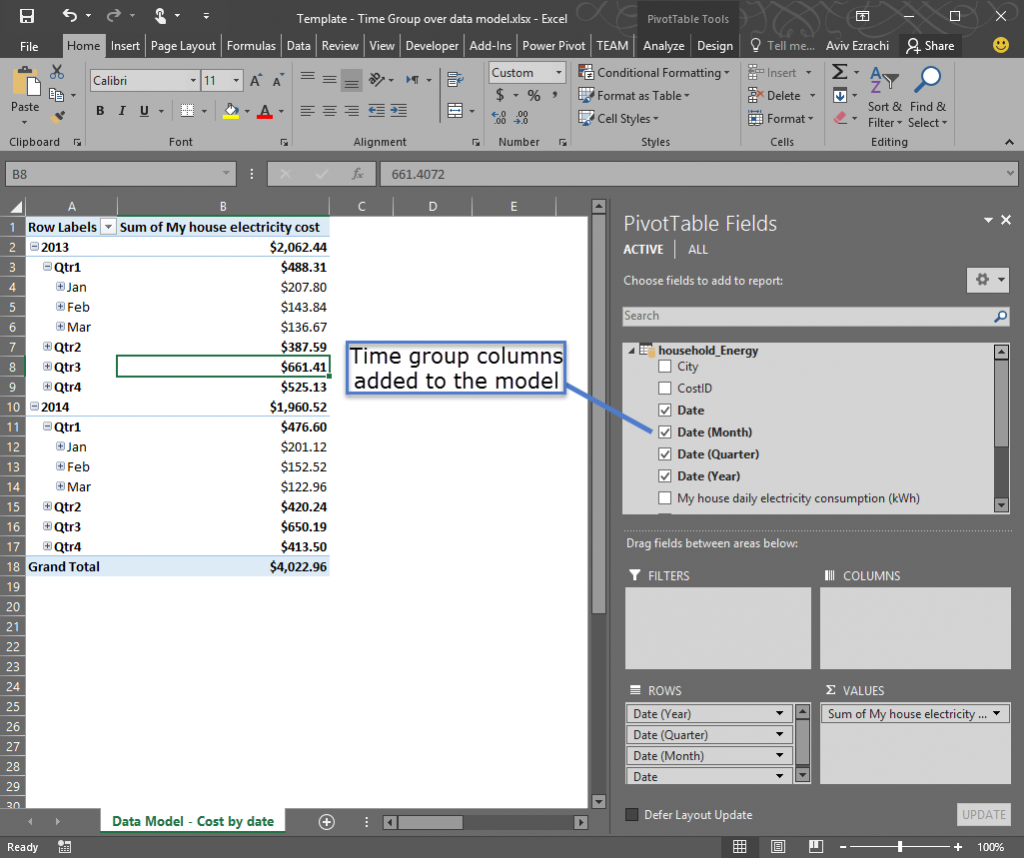
PivotTable grouping is used frequently by customers in many business scenarios. Implementing grouping for Data Model PivotTables allows for grouping to be used in conjunction with the power of the xVelocity engine and is a key feature for making Data Model PivotTables a replacement for native ones in the future. When used in a data model PivotTable, Time grouping adds relevant Date/Time columns such as Date (Year), Date (Quarter) and Date (Month) to the grouped table in the model; these columns could then be reused with other user endpoints of the data model, such as PowerView and Power BI.

Time grouping columns in the model.

The Date/Time columns are automatically added according to the Data column date/time granularity. For example, if the date data is in days and is for more than a year’s duration, then the added grouping columns would be for months, quarters and years.

Once the Date/Time columns are added to the model, not only can you analyze your data over the different time granularities it entitles, but you may also find additional insights. For example, to get a monthly year-over-year comparison of your data, drag the Date (Year) column over from the ROWS drop zone to the COLUMNS drop zone while keeping only the Date (Months) column in the ROWS drop zone.

Auto-grouping for a data model PivotTable also means that for the first time in Excel you are able to aggregate data larger than one million rows.

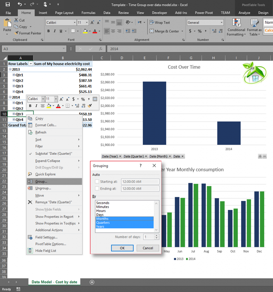
Right-click Group and Group dialog.

Changing the Group columns is always possible through the usual user interface. In the PivotTable, right-click the Date column and select Group.

The Group dialog is where you can define other columns to be added or removed from the time group. You may have noticed that “Starting at/Ending at” and “Number of days” are greyed out; this is because we do not support these settings for data model PivotTables.

Don’t like automatic grouping? Undo it just like you would any other applied change. The first undo (Ctrl+Z) removes the auto-added columns from the ROWS drop zone. The second undo removes the newly added columns from the model, so you are back at square one. In case these columns are already used in another PivotTable, then they will not be deleted from the model. Right-click Ungroup… is also supported and will act as if you have done the two undo operations, removing the group fields from the drop zones and the model. You can also turn off automatic time grouping.

When the model already contains a “Date Table,” we do not want to do time grouping, since the “Date Table” includes all required date columns already. So when building a PivotTable and dragging a Date column from a “Date Table” from the data model, automatic grouping would not apply.

PivotChart drill-down buttons

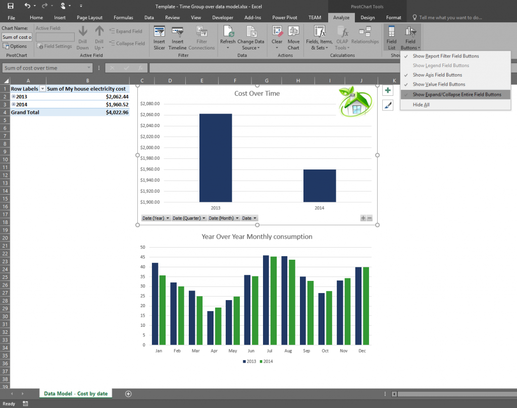
PivotCharts have always supported a double-click on a chart element to do a drill-down to the next level of the selected element. This is the same as clicking the plus sign on the PivotTable collapsed level. A tougher job is when you want to expand all objects in the PivotTable to the next level. This is where the newly added PivotChart drill-down buttons come in handy, as clicking the + (plus) or – (minus) buttons allow you to drill down to the next level of all elements in the charts with a single click.

This functionality applies to any hierarchy or any set of columns in the ROWS drop zone of the PivotChart.

When you open a PivotTable created on a previous version of Excel, you will not see the new drill-down buttons until you enable them on the Analyze ribbon. It is also possible to remove these buttons from a chart created in Excel 2016.

Toggle viewing of PivotChart field buttons.

Reuse of time group fields in Power BI

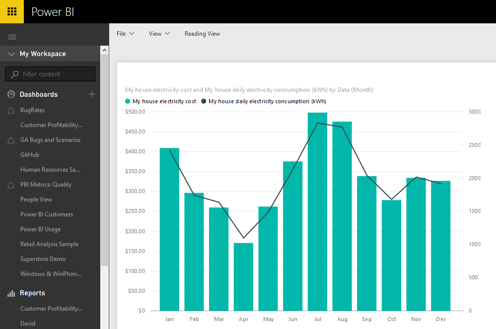
The new Date columns really come in handy in Power BI. One noticeable value to users is that the Month column added to the data model through the Automatic Grouping in Excel is calendar ordered (Jan, Feb, Mar…).

The new Date columns put to use in PowerBI.com.